William_Potter
The long-term return forecast for the World Market Index (GMI) continued to ease in January, dipping to an annualized 6.6% complete return, based mostly on the typical of three fashions (outlined beneath). GMI is a market value-weighted portfolio that holds all of the major asset classes (besides money) by way of a set of ETF proxies. At present’s revised efficiency estimate marks one other fractionally decrease forecast vs. the previous month’s outlook.
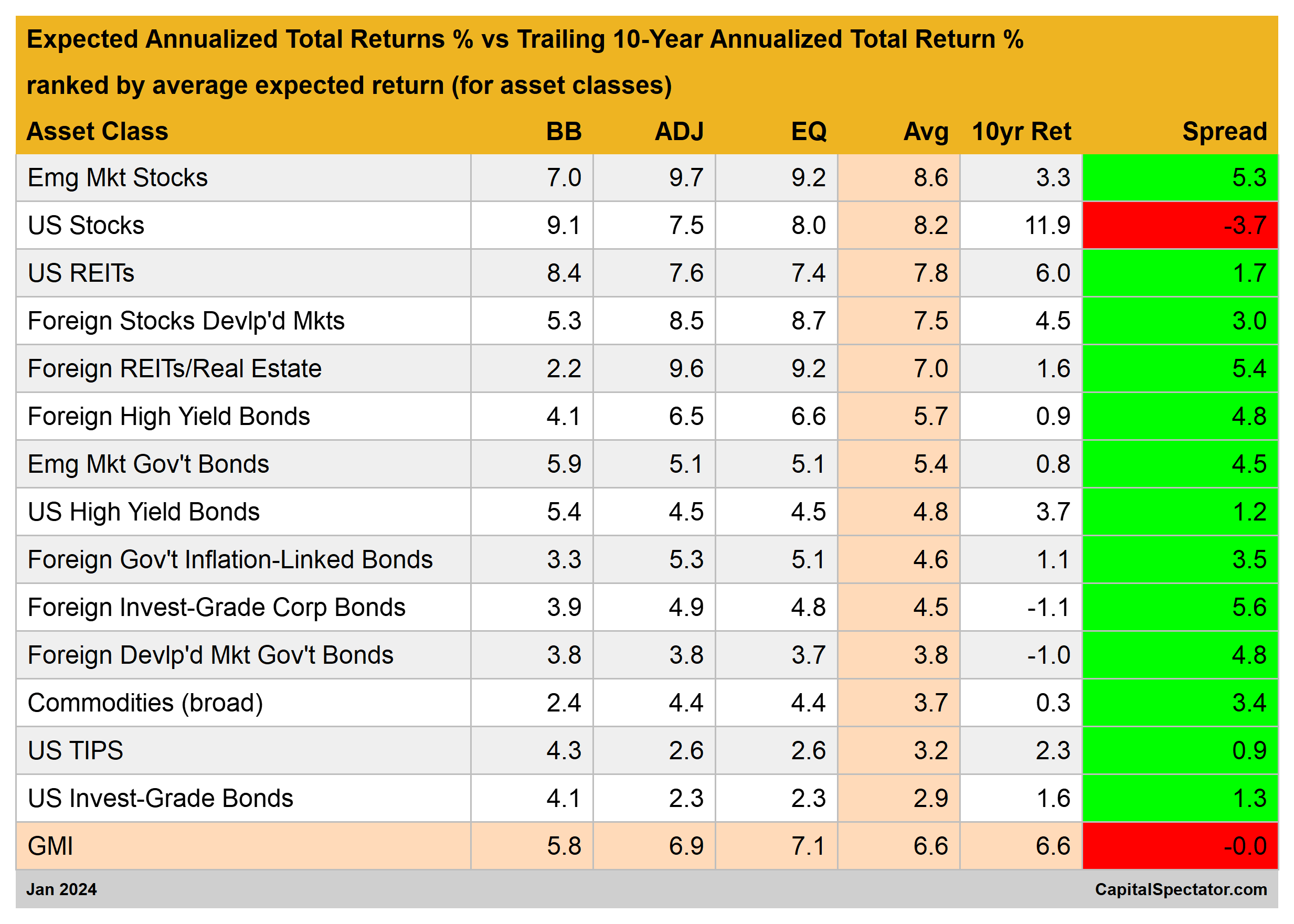
As soon as once more, the ex-ante return for US shares is the conspicuous outlier: the typical return forecast is effectively beneath the trailing 10-year efficiency. American equities, in sum, are anticipated to ship materially decrease returns relative to the previous decade. In contrast, the remainder of the key asset lessons replicate efficiency forecasts above their respective trailing 10-year outcomes. In the meantime, GMI is at the moment projected to generate a return that is according to its trailing 10-year efficiency of 6.6%.
GMI represents a theoretical benchmark of the optimum portfolio for the typical investor with an infinite time horizon. On that foundation, GMI is helpful as a start line for customizing asset allocation and portfolio design to match an investor’s expectations, goals, threat tolerance, and so on. GMI’s historical past means that this passive benchmark’s efficiency is aggressive with most energetic asset allocation methods, particularly after adjusting for threat, buying and selling prices, and taxes.
It is probably that some, most, or presumably the entire forecasts above will probably be vast off the mark to a point. GMI’s projections, nevertheless, are anticipated to be considerably extra dependable vs. the estimates for its elements. Predictions for the particular markets (US shares, commodities, and so on.) are topic to higher volatility and monitoring error in contrast with aggregating the forecasts into the GMI estimate, a course of that will cut back some errors by time.
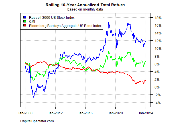
For context on how GMI’s realized complete return has developed by time, think about the benchmark’s observe report on a rolling 10-year annualized foundation. The chart beneath compares GMI’s efficiency vs. the equal for US shares and US bonds by final month. GMI’s present return for the previous ten years is 6.6%, which is reasonably above the current low for this time window.
Here is a short abstract of how the forecasts are generated and definitions of the opposite metrics within the desk above:
BB: The Constructing Block mannequin makes use of historic returns as a proxy for estimating the longer term. The pattern interval used begins in January 1998 (the earliest accessible date for all of the asset lessons listed above). The process is to calculate the danger premium for every asset class, compute the annualized return, after which add an anticipated risk-free price to generate a complete return forecast. For the anticipated risk-free price, we’re utilizing the newest yield on the 10-year Treasury Inflation-Protected Safety (TIPS). This yield is taken into account a market estimate of a risk-free, actual (inflation-adjusted) return for a “safe” asset – this “risk-free” price can be used for all of the fashions outlined beneath. Notice that the BB mannequin used right here is (loosely) based mostly on a strategy initially outlined by Ibbotson Associates (a division of Morningstar).
EQ: The Equilibrium mannequin reverse engineers anticipated return by the use of threat. Reasonably than attempting to foretell return instantly, this mannequin depends on the considerably extra dependable framework of utilizing threat metrics to estimate future efficiency. The method is comparatively sturdy within the sense that forecasting threat is barely simpler than projecting return. The three inputs:
* An estimate of the general portfolio’s anticipated market value of threat, outlined because the Sharpe ratio, which is the ratio of threat premia to volatility (normal deviation). Notice: the “portfolio” right here and all through is outlined as GMI.
* The anticipated volatility (normal deviation) of every asset (GMI’s market elements).
* The anticipated correlation for every asset relative to the portfolio (GMI).
This mannequin for estimating equilibrium returns was initially outlined in a 1974 paper by Professor Invoice Sharpe. For a abstract, see Gary Brinson’s rationalization in Chapter 3 of The Portable MBA in Investment. I additionally evaluate the mannequin in my ebook Dynamic Asset Allocation. Notice that this technique initially estimates a threat premium after which provides an anticipated risk-free price to reach at complete return forecasts. The anticipated risk-free price is printed in BB above.
ADJ: This system is equivalent to the Equilibrium mannequin (EQ) outlined above with one exception: the forecasts are adjusted based mostly on short-term momentum and longer-term imply reversion elements. Momentum is outlined as the present value relative to the trailing 12-month shifting common. The imply reversion issue is estimated as the present value relative to the trailing 60-month (5-year) shifting common. The equilibrium forecasts are adjusted based mostly on present costs relative to the 12-month and 60-month shifting averages. If present costs are above (beneath) the shifting averages, the unadjusted threat premia estimates are decreased (elevated). The formulation for adjustment is just taking the inverse of the typical of the present value to the 2 shifting averages. For instance: if an asset class’s present value is 10% above its 12-month shifting common and 20% over its 60-month shifting common, the unadjusted forecast is lowered by 15% (the typical of 10% and 20%). The logic right here is that when costs are comparatively excessive vs. current historical past, the equilibrium forecasts are lowered. On the flip facet, when costs are comparatively low vs. current historical past, the equilibrium forecasts are elevated.
Avg: This column is a straightforward common of the three forecasts for every row (asset class)
10yr Ret: For perspective on precise returns, this column exhibits the trailing 10-year annualized complete return for the asset lessons by the present goal month.
Unfold: Common-model forecast much less trailing 10-year return.
Editor’s Notice: The abstract bullets for this text had been chosen by Looking for Alpha editors.